Working with CoolProp in Excel (and vba)

CoolProp is a very useful package for the calculation of the physical (transport and thermodynamic) properties of pure fluids and mixtures. Usually, I call it from Julia or Python, but when it comes to communication with colleagues, they often prefer an excel file. I must confess, excel is not my cup of tea and I constantly make mistakes. Even when everything works fine, I suddenly run into a problem that can be solved way easier using a Python/Julia script. I'm not saying excel is a weak or bad tool; I'm just saying other tools are better!
Few months ago, I calculated the pressure drop of a CO2 transport pipeline and the amount of compression work that is required for the gas transport. For the pressure drop, I used the Weymouth correlation. I first calculated the isentropic work of a compressor and then divided it by the mechanical efficiency of a centrifugal compressor to estimate the real power requirement. I assumed a multi-stage compressor with inter-stage cooling and a maximum compression ratio of three to three and a half. This is something that can be probably done in an excel sheet, but can be done much easier with a few lines of code. The same hold for the calculation pf pressure drop. Gas is compressible, and as the pressure drops in the pipeline, gas expands and it linear velocity increases. Therefore, the pressure drop needs to be calculated in short segments of the pipe, where we can assume the physical properties of the gas phase are constant. This segment based calculations although fits into an excel sheet, is not something that we need to see in detail. We are only interested in the pressure drop in the whole pipeline, not in every little segment.
This encouraged me to overcome my excel-phobia and dive into it by writing two macros for the calculation of pressure drop in a gas pipeline and the power requirement in a compressor. I did not document the procedure, but I try my best to repeat it here with all the details. Here's the (main part of) formulation: $$W_{comp} = H(T(S_{out}, p_{out}), p_{out}) - H(T_{in}, p_{in})$$ The above equation means that the compression process is reversible, so we can calculate the temperature of the compressed gas, assuming that its entropy is equal to the entropy of the input gas stream.

Requirements

A windows machine (or a windows virtual machine like mine) with Microsoft Excel installed.

Step 1: install CoolProp for Windows

Go to this web page and download the CoolProp installer (a file called CoolProp_v6.1.0.0.exe). I worked with version 6.1.0. You can alternatively download the latest version from here. I installed it with all the default settings. You may want to do the same.

Step 2: test your installation

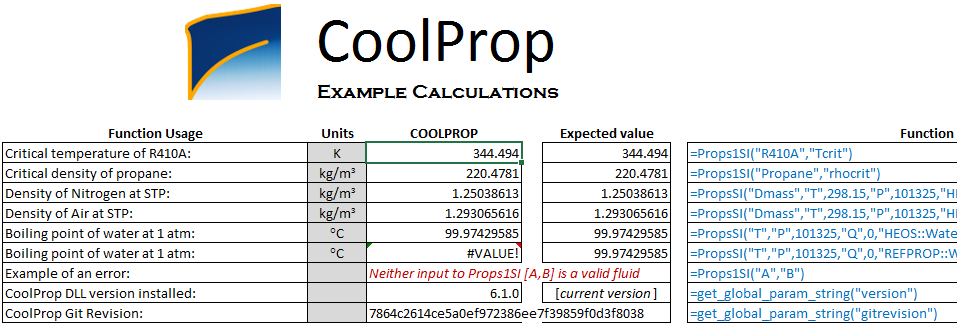
CoolProp installer copies a test excel file called TestExcel.xlsx on your desktop. Open it and make sure that it works fine. By fine, I mean this screen-shot: coolprop sample calculation excel If it doesn't work and you cannot see the numbers, go to the Installation sheet in the same excel file and follow the instructions.
Step 3: start writing a VBA function

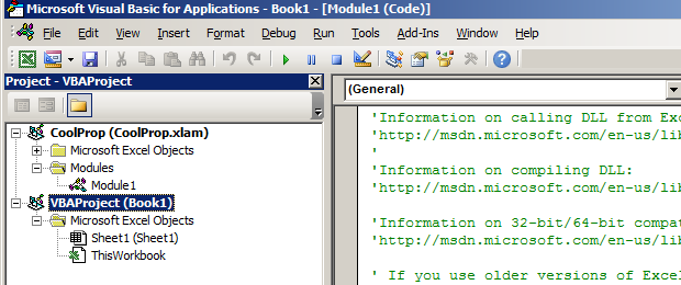
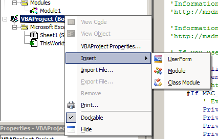
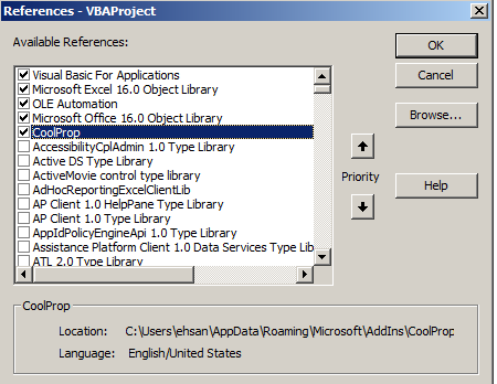
Create a new excel workbook. Then press Alt + F11 to open the Microsoft Visual Basic for Applications. You will see something like this: visual basic excel coolprop Right click on VBAProject (Book1) and choose Insert -> Module: new-module-vba-coolprop Before writing your new function in the module, you need to tell excel that you are going to call CoolProp functions. To do that, go to Tools -> References... and check the box next to CoolProp like the following and then press OK. reference coolprop vba
Step 4: Write your function

This is the function I have written for the calculation of the compression work. The inputs are number of compression stages (n_stage), the temperature in Kelvin after the inter-cooling stage (T_comp), input and output pressure for each compressor in Pascal (p_in and p_out), and gas_type which is the name of the fluid, e.g., "CO2". Copy and paste the function into your new module.

Function comp_work(n_stage, T_comp, p_in, p_out, gas_type)
w_min_transport = 0#
comp_ratio = Exp(Log(p_out / p_in) / n_stage)
p_comp = p_in
p_comp_next = comp_ratio * p_comp
  For i = 1 To n_stage
    S_in = CoolProp.PropsSI("SMOLAR", "T", T_comp, "P", p_comp, gas_type) ' molar entropy J/(mol.K)
    H_in = CoolProp.PropsSI("HMOLAR", "T", T_comp, "P", p_comp, gas_type) ' molar enthalpy J/mol
    ' find the output T for isentropic compressor
    ' S_in-CoolProp.PropsSI("SMOLAR", "T", T_comp, "P", p_out, gas_type)
    T_out = CoolProp.PropsSI("T", "SMOLAR", S_in, "P", p_comp_next, gas_type)
    H_out = CoolProp.PropsSI("HMOLAR", "T", T_out, "P", p_comp_next, gas_type) ' molar enthalpy J/mol
    w_min_transport = w_min_transport + H_out - H_in ' J/mol
    p_comp = p_comp_next
    p_comp_next = p_comp * comp_ratio
  Next i
comp_work = w_min_transport
End Function

Step 5: test your new function

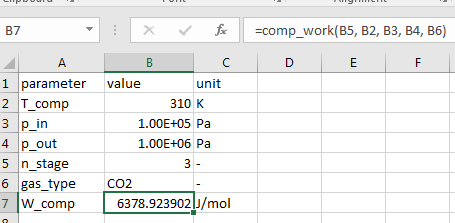
The (macro-enabled) excel file contains the vba code and a simple test, can be downloaded here; the final results should look like this: test excel vba coolprop
Starting with Reaktoro

I recently heard about the Reaktoro project, which is a platform for the fast calculation of geochemical reactions (both equilibrium and kinetics). I'm working mostly with the adsorption reactions, so I was not interested at the beginning although the code is very polished, clean, and readable even for me with a tiny knowledge of C++. At the end the Python interface and the Helgeson-Kirkham-Flowers (HKF) equation of state tempted me to give it a try. I followed the installation procedure here and it went very well on my Linux Mint machine. The Python package is installed in the /usr/local/lib/python2.7/site-packages/ which is not in the python path. You need to add it manually:

In [1]:
import sys
sys.path.append("/usr/local/lib/python2.7/site-packages/")

Then I looked at the Python examples and demos and found the answer to my question: calculation of (partial molar) Gibbs energy and the equilibrium constants for some electrolyte reactions, using the HKF EOS and a beautiful scripting language. It even convinced me to create a bitbucket account! As an example, the following code (that is a modified version of a Reaktoro example) is how the equilibrium constant for a reaction can be calculated:

In [2]:
from reaktoro import *
from numpy import *
import matplotlib.pyplot as plt
In [3]:
database = Database("supcrt98.xml")
thermo = Thermo(database)

I am interested in the equilibrium constant of the following reaction:
$$ CaOH^+ + SO_4^{-2} = CaSO_4 + OH^-$$ I tried different way of writing this reaction and finally the following version worked:

In [4]:
reac1 = 'CaOH+ + SO4-- = CaSO4(aq) + OH-'
T = 300 # K
p = 1e5 # Pa
R = 8.3144598 # J/(mol.K)
thermo.lnEquilibriumConstant(T, p, reac1).val
Out[4]:
2.145092126874757

Let's do the calculation by using the basic relation $$\ln K_{eq} = \frac{-\Delta_r G}{RT} $$

In [5]:
dgrt = thermo.standardPartialMolarGibbsEnergy(T, p, 'CaSO4(aq)').val+ \
thermo.standardPartialMolarGibbsEnergy(T, p, 'OH-').val- \
thermo.standardPartialMolarGibbsEnergy(T, p, 'SO4--').val- \
thermo.standardPartialMolarGibbsEnergy(T, p, 'CaOH+').val
-dgrt/R/T
Out[5]:
2.1450927202641066

There is a small difference between the two values that I guess is due to the difference between the number of significant digits that I have used for the universal gas constant. Otherwise, everything works great, and the values are in agreement with what I have previously calculated myself.

Van't Hoff equation

Let's do something interesting. We know from Van't Hoff equation that $$\frac{\text{d}\ln K_{eq}}{\text{d}\frac{1}{T}} = -\frac{\Delta_r H}{R}.$$ It means that if I plot $\ln K_{eq}$ versus $\frac{1}{T}$, I get (almost) an straight line with a slope of $-\frac{\Delta_r H}{R}$. Let's do the calculations in Reaktoro:

In [6]:
T_range = linspace(25+273.15, 80+273.15, 10)
ln_keq = []
for T in T_range:
    ln_keq.append(thermo.lnEquilibriumConstant(T, p, reac1).val)
plt.plot(1/T_range, ln_keq)
plt.xlabel("1/T [1/K]")
plt.ylabel("ln(K_eq)")
plt.show()

Compare the results

We can calculate the enthalpy of reaction in different temperatures in Reaktoro and compare it with the approximate value that is the slope of the above line multiplied by -R. Let's do the calculation and plot the results:

In [7]:
dh_fit  = -polyfit(1/T_range, ln_keq, 1)[0]*R
dh_calc = []
for T in T_range:
    dh_calc.append(thermo.standardPartialMolarEnthalpy(T, p, 'CaSO4(aq)').val+ \
    thermo.standardPartialMolarEnthalpy(T, p, 'OH-').val- \
    thermo.standardPartialMolarEnthalpy(T, p, 'SO4--').val- \
    thermo.standardPartialMolarEnthalpy(T, p, 'CaOH+').val)
plt.plot(T_range, dh_calc, label = "HKF")
plt.plot(T_range, ones(T_range.size)*dh_fit, label = "Van't Hoff")
plt.legend()
plt.xlabel("T [K]")
plt.ylabel("\Delta H [J/mol]")
plt.show()

In my opinion, it is very important for a software to enable the user to do the very basic stuff as Reaktoro helped me to do the above calculations. I still miss a few functionalities in Reaktoro: oxidation/reduction reaction and ion exchange/surface complexation models. Fortunately, Reaktoro is under active development and the new features will appear soon.

Calling Phreeqc from Julia: a tutorial

In this post, I'm going to show how we can call Phreeqc from Julia to calculate the solubility of minerals in a solution. The workflow is very useful specially when one wants to conduct a sensitivity analysis and plot the results. Here is my workflow:

  • Create a Phreeqc input file in Julia
  • Save it to a text file
  • Call Phreeqc from Julia to run the created input file
  • Read the results from the output file created by Phreeqc
  • Plot the results

If you are on windows, you need to add phreeqc to the path so you can call it from the command line.

create a Phreeqc simulation file

The following string is a phreeqc input file that mixes 10.0 moles of anhydrite in 1 kg of demineralized water at 50 degree Celsius and 250 atm, and writes the molality of Ca ion in the aqueous solution to an output file named anhydrite_solubility.csv:

SOLUTION 1 Pure water
    pH      7.0
    temp    50.0
    pressure  10
EQUILIBRIUM_PHASES 1
    Anhydrite       0.0     10.0
SELECTED_OUTPUT
    -file   anhydrite_solubility.csv
    -reset false
    -totals     Ca
END

You can save this code in a file names e.g., anhydrite_sol.phr, and run it by

phreeqc anhydrite_sol.phr

if you have phreeqc installed and in your path. In windows, you can download phreeqc for windows and run it.

Sensitivity analysis

My purpose here is to study the effect of thermodynamic models and databases, temperature, and pressure on the predicted solubility of anhydrite in water. It can be done manually, but I like to do it automatically from a Julia script. You ca do it in Matlab or any other tools of your choice.

The workflow

We first create the Phreeqc input file as an string in Julia. Then, we save that script into a file and call phreeqc to run it. We save the results in an output file and read it in Julia. Finally we plot the results. The following script shows how this can be done in Julia. We need to use the packages PyPlot for visualization and DataFrames for reading the output file.

In [1]:
using PyPlot, DataFrames
In [2]:
T_min = 25.0     # degC minimum temperature
T_max = 100.0    # degC maximum temperature
p_atm = 250       # atm pressure
T_range = collect(linspace(T_min, T_max, 20))
data_base = ["phreeqc.dat", "pitzer.dat"]
for db in data_base
    anhydrite_sol = zeros(0)
    for T in T_range
        phreeqc_input =
        """
        DATABASE /usr/local/share/doc/phreeqc/database/$db
        SOLUTION 1 Pure water
            pH      7.0
            temp    $T
            pressure  $p_atm
        EQUILIBRIUM_PHASES 1
            Anhydrite       0.0     10.0
        SELECTED_OUTPUT
            -file   anhydrite_solubility.csv
            -reset false
            -totals     Ca
        END
        """
        # save it to a file
        ph_file=open("phreeqc_input_file", "w")
        write(ph_file, phreeqc_input)
        close(ph_file)
        # run it
        run(`phreeqc phreeqc_input_file`)
        # read the results
        ph_res=readtable("anhydrite_solubility.csv", separator = ' ')
        # plot the results
        push!(anhydrite_sol, ph_res[:Ca][end])
    end
    IJulia.clear_output()
    plot(T_range, anhydrite_sol)
end
legend(data_base)
xlabel("Temperature(C)")
ylabel("Anhydrite solubility [mol/kgw]");

You probably need to change the path to the Phreeqc databeses in line 11 of the above code. Play with the value of pressure and see what happens. It is truely fascinating that increasing pressure can affect the solubility that much. Don't forget that it can only be captured by the Pitzer model in Phreeqc.
There is another way of calling Phreeqc from Julia that I will discuss later.

Two phase flow and capillary pressure: part I

Capillary pressure

Imagine a very thin glass tube filled with water. If the tube is thin enough, water likes to stay in the tube. You have to blow in the tube to push it out. In other words, to replace water that wets the glass with air, we need to push air into the tube. The amount of pushing that you need for air to go through is called capillary pressure. Its value, which is defined as $$p_c=p_{air}-p_{w},$$ is related to the water-air surface tension, contact angle, and tube diameter with the following relation: $$p_c=\frac{\gamma_{w-air}\cos(\theta)}{r}.$$
In Petroleum Engineering, capillary pressure has the same definition: $$p_c=p_{nw}-p_w,$$ where subscripts nw and w denote 'non-wetting' and 'wetting' phases respectively. However, a porous medium is made of many tubes with different sizes. Therefore, when we want to blow water out of it, the amount of required 'pushing' depends on the number of tubes that are already filled with water (or the wetting phase). In other words, the capillary pressure depends on the 'wetting-phase saturation'. If we assume the average tube radius can be defined by \(\sqrt{k/\phi}\), with k permeability and \(\phi\) porosity, we can write the capillary pressure in a porous medium as $$p_c=J(S_w)\frac{\gamma_{w-nw}\cos(\theta)}{\sqrt(k/\phi)}$$ Clearly, someone has done it years ago, and therefore the function J is conveniently called the Leverett J-function.

The J-function

Let's think about the porous medium as a bundle of water-wet tubes with different diameters. First the tubes are filled with water, i.e., the water saturation is one. When we start blowing air into the tubes to push water out, at the beginning the minimum resistance is in the tube with the maximum diameter (see the definitions in the previous section). The amount of pressure that is required to push water out of the largest tube is called the entry capillary pressure. Then one by one we push water out of the thinner tubes. I always wanted to try this for myself. Why not here?

Capillary pressure for a bundle of tubes

The following code plots the capillary pressure versus water saturation for the drainage and imbibition processes. I use some assumptions for the estimation of dynamic contact angle, to take into account the hysteresis.

In [1]:
using PyPlot
In [2]:
r_min=1e-7 # [m]
r_max=1e-6 # [m]
r=collect(linspace(r_min, r_max, 100))
gama_gw=0.072 # [N/m]
teta=deg2rad(30.0)
teta_min=deg2rad(5.0)
teta_max=deg2rad(110.0)
# advance (imbibe)
# r_max: teta
# r_min: teta_max
teta_imb=(teta_max-teta)/(r_max^2-r_min^2)*(r.^2-r_min^2)+teta
# recede (drain)
# r_max: teta
# r_min: teta_min
teta_drain=(teta-teta_min)/(r_max^2-r_min^2)*(r.^2-r_min^2)+teta_min
v=π*r.^2
v_tot=sum(v)
s=cumsum(v)/v_tot
p_drain=gama_gw*cos(teta_drain)./r
p_imb=gama_gw*cos(teta_imb)./r
plot(s,p_drain, s, p_imb)
xlabel(L"S_w")
ylabel(L"P_c [Pa]")
grid()
legend(["Drainage", "Imbibition"]);

Other facts

The above curves were obtained with a few simplistic assumptions. There are other very important concepts, e.g., connate water saturation are not taken into account. I am not going to improve the above model. However, I will write about the imbibition and drainage in porous media in the next part of this post.

Why am I doing this?

No one has asked me this question yet, but I'm going to answer it anyway. I'm not writing anything new, or something that you cannot find in the standard textbook. I have two objectives: to write more in English, and to try to simplify things in case I want to teach it one day in near future.

A nanoparticle at the gas-liquid interface: using Sympy

My post-doc research was about nanoparticle-stabilized foam for enhanced oil recovery. Foam is usually generated by blowing gas into a surfactant-water solution. Surfactant molecules go to the gas-liquid interface and prevent (or slow down) the drainage (sort of) and collapse of the liquid films. Mixed-wet particles act like surfactants. When they go to the interface, the amount of energy that is required to move them back to the gas or liquid phase is a few orders of magnitude higher than the thermal energy of the particles, which makes the liquid film generated by nanoparticles quite stable. There is a classic relation for the desorption energy (or the amount of energy to move the particles from the interface to a bulk phase). Few weeks ago, I was discussing the stability of nanoparticle-foam with a colloid-chemistry Professor who shortly visited our department during his trip to Delft. He pointed out that this relation may be wrong, as it seems that it does not consider all the gas-liquid, gas-solid, and liquid-solid interactions. I tried to derive the equation for myself, and I thought it is a good time to play with Sympy and SymPy.jl. First, install sympy by

sudo pip install sympy

and install SymPy in Julia by

Pkg.add("SymPy")

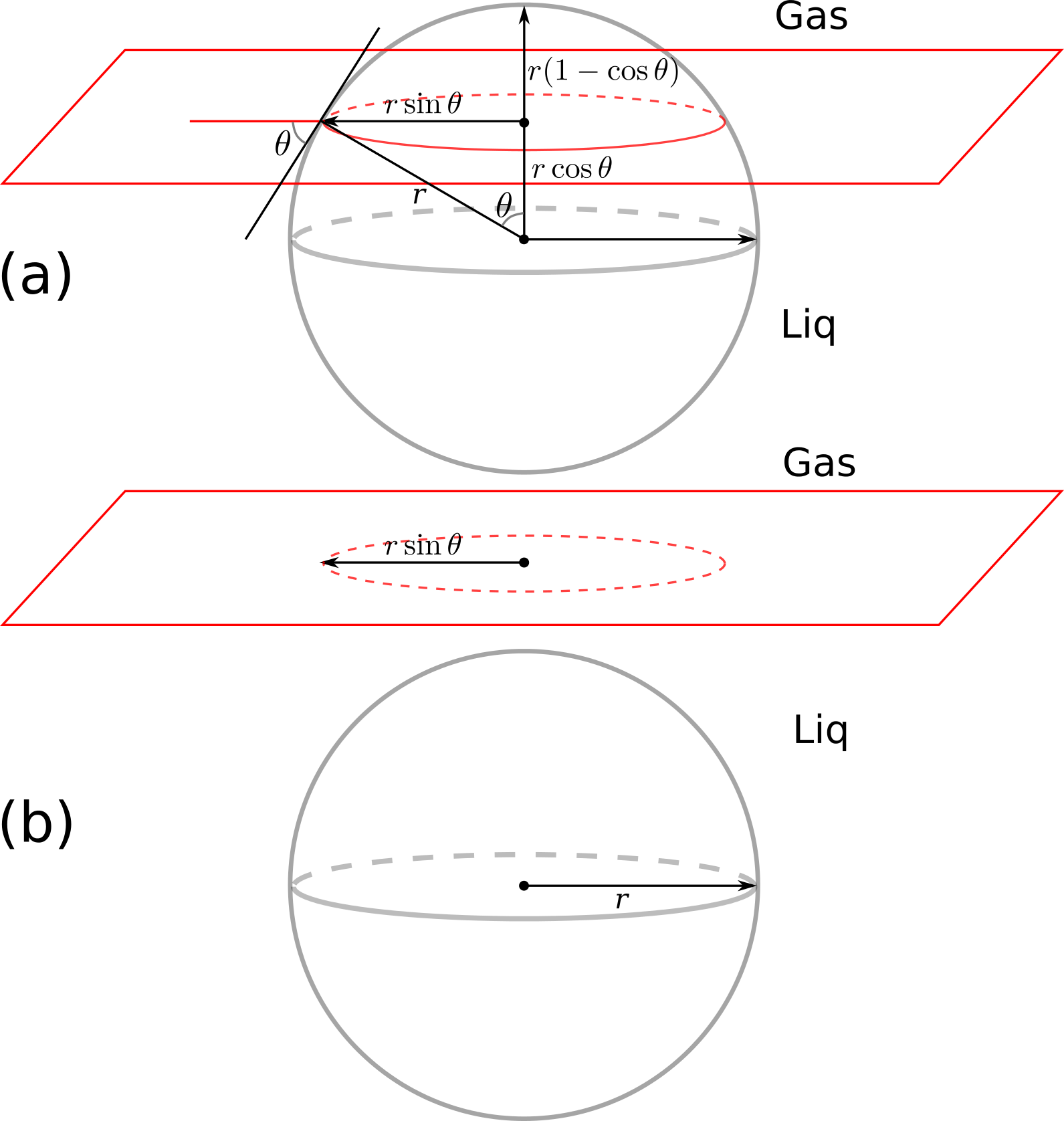
Now have a look at the following figures: part (a) shows the particle at the interface and part (b) shows the particle removed from the interface to the aqueous phase:

nanoparticle at the interface

In [1]:
using SymPy

First, we define all the symbolic variables:

In [2]:
gama_gw, gama_sw, gama_sg, r, teta=symbols("gamma_gw, gamma_sw, gamma_sg, r, theta")
Out[2]:
(gamma_gw,gamma_sw,gamma_sg,r,theta)

The interfacial energy in part (a) is calculated by surface area multiplied by the inerfacial energy of the respective phases:

In [3]:
E1=2*PI*r*r*(1-cos(teta))*gama_sg+(4*PI*r^2-2*PI*r*r*(1-cos(teta)))*gama_sw
Out[3]:
$$2 \pi \gamma_{sg} r^{2} \left(- \cos{\left (\theta \right )} + 1\right) + \gamma_{sw} \left(- 2 \pi r^{2} \left(- \cos{\left (\theta \right )} + 1\right) + 4 \pi r^{2}\right)$$

We do the same for the part (b) of the figure, where the particle is in the liquid phase:

In [4]:
E2=gama_sw*4*PI*r^2+gama_gw*PI*(r*sin(teta))^2
Out[4]:
$$\pi \gamma_{gw} r^{2} \sin^{2}{\left (\theta \right )} + 4 \pi \gamma_{sw} r^{2}$$

The difference between the total interfacial energy of state (a) and (b) is calculated by:

In [5]:
dE=E2-E1
Out[5]:
$$\pi \gamma_{gw} r^{2} \sin^{2}{\left (\theta \right )} - 2 \pi \gamma_{sg} r^{2} \left(- \cos{\left (\theta \right )} + 1\right) + 4 \pi \gamma_{sw} r^{2} - \gamma_{sw} \left(- 2 \pi r^{2} \left(- \cos{\left (\theta \right )} + 1\right) + 4 \pi r^{2}\right)$$

We can simplify the above equation by using the Young-Dupre equation, which reads $$\gamma_{sg}=\gamma_{sw}+\gamma_{gw}\cos(\theta)$$

In [6]:
dE2=subs(dE, gama_sg, gama_sw+gama_gw*cos(teta))
Out[6]:
$$\pi \gamma_{gw} r^{2} \sin^{2}{\left (\theta \right )} + 4 \pi \gamma_{sw} r^{2} - \gamma_{sw} \left(- 2 \pi r^{2} \left(- \cos{\left (\theta \right )} + 1\right) + 4 \pi r^{2}\right) - 2 \pi r^{2} \left(\gamma_{gw} \cos{\left (\theta \right )} + \gamma_{sw}\right) \left(- \cos{\left (\theta \right )} + 1\right)$$

Now we simplify the equation in sympy:

In [7]:
simplify(dE2)
Out[7]:
$$\pi \gamma_{gw} r^{2} \left(\cos{\left (\theta \right )} - 1\right)^{2}$$

Voila! Normally the equation is reported as $$\Delta E=\pi \gamma_{gw} r^2 (1-\cos(\theta))^2,$$ which is identical to what we obtained above. Have a look at this tutorial to learn more about symbolic mathematics in Python and Julia.

FVTool in Octave: the new classdef

The new octave version was recently released and I was excited to test the new classdef, to use my Matlab FVTool with the same functionality in the free (as in free speech and free coffee) Octave. In the process of rewriting the code, I use the design of JFVM.jl. The good news is that now the syntax for JFVM and FVTool are almost identical, except the differences between the languages. The other good news is that now the package supports nonuniform grids. I have already used that feature in a paper (well, an appendix of a paper). The bad news is that the new API is not compatible with the previous version of FVTool. I have updated all the examples to the new API. If you like the older version, please use this link to download it. The main change in the new version is that now CellVariable and FaceVariable are new objects, with a MeshStructure field, and a value, or xvalue, yvalue, and zvalue fields. and therefore you don't need to send MeshStructure as an argument to the discretization and Calculus functions.
One other small change is that I had to disable a function call in the visualization routines, viz. alpha. If you are in Matlab and you like to make your visualization fancier by adding a bit of transparency, consider enabling this function in the visualization routines. The visualization is very basik anyway. I will think about a better way to export the results to other visualization packages for the future versions.
Let's see the code in action:

In [2]:
addpath('/home/ali/MyPackages/FVTool')
FVToolStartUp()
Out[2]:
AGMG 3.x linear solver is NOT available.
warning: PVTtoolbox could not be found; Please run PVTinitialize.m manually
FiniteVolumeToolbox has started successfully.
In [5]:
% create a nonuniform mesh
x=[0,0.1, 0.2, 0.25, 0.4, 0.42, 0.43, 0.6, 0.75, 0.9, 0.91, 0.92, 0.95, 1.0];
m=createMesh1D(x);
m3=createMesh3D(x,x,x);
m
Out[5]:
m =

<object MeshStructure>

As you can see, m is not of type struct anymore. I have used classdef to define its own object type, in this case MeshStructure.

In [10]:
D=createCellVariable(m, 1.0);
D_face=arithmeticMean(D); # no need to send the mesh variable to the function
disp(D)
Out[10]:
<object CellVariable>

You can see that D is now a CellVariable object, and the mesh over which it is defined is stored in:

In [11]:
D.domain
Out[11]:
ans =

<object MeshStructure>

Let's continue and solve a diffusion equation over the 3D domain:

In [13]:
D=createCellVariable(m3, 1.0);
D_face=arithmeticMean(D);
BC=createBC(m3);
BC.left.a(:)=0; BC.left.b(:)=1.0; BC.left.c(:)=1.0;
BC.right.a(:)=0.0; BC.right.b(:)=1.0; BC.right.c(:)=0.5;
[Mbc, RHSbc]=boundaryCondition(BC);
Md=diffusionTerm(D_face);
c=solvePDE(m3, Md+Mbc, RHSbc);
visualizeCells(c)
Out[13]:

I'll come back with more interesting cases in the FVT blog.

Install Octave 4.0 on Mint 17.1/Ubuntu 14.04

Simple method

In a terminal, write

sudo add-apt-repository ppa:octave/stable
sudo apt-get update
sudo apt install octave

That's it!

Hard alternative

Octave version 4.0 is out, and the good news is that it has a classdef feature similar to Matlab. I will soon use it to update my FVTool so that it can be used with all functionalities in Octave as well.
The problem is that it takes a while before the new version of Octave comes to the software center of Ubuntu. I decided to compile and build it, although I've never had a good experience with building tools from source. This time however it worked however without any issue on my laptop and my pc. I used the procedure I found here. I had to install some more libraries on my Mint 17.1 operating system.
First, install these dependencies:

sudo apt-get install gawk gfortran gperf flex libbison-dev libqhull-dev libglpk-dev libcurl4-gnutls-dev libfltk1.3-dev librsvg2-dev libqrupdate-dev libgl2ps-dev libosmesa6-dev libarpack2-dev libqscintilla2-dev libreadline-dev bison icontool llvm-dev libfftw3-dev libhdf5-serial-dev openjdk-7-jdk transfig  libgraphicsmagick++1-dev libsndfile1-dev

Then, download the octave source code for version 4.0.0 from here, and extract it. Go to the new octave-4.0.0 forlder, and in a terminal window type

./configure --enable-jit
make
sudo make install

It takes a while, so go and pour a nice cup of coffee for yourself. If you get any error after running ./configure, find the missing dependencies here.
If the installation is successful, run octave by typing octave. It should launch the user interface of octave which is enabled by default in this version.
One other good news is that now you can run octave in a Jupyter notebook, by installing octave kernel and oct2py:

sudo pip install oct2py
sudo pip install octave_kernel

It is still not possible to use octave kernel. Go to /usr/local/bin and type

ls -la

You will see that octave is linked to the octave-4.0.0. You need to unlink octave and create a symbolic link to the octave command line interface or octave-cli. In the terminal window, type

sudo unlink octave
sudo ln -s /usr/local/bin/octave-cli octave

Now your octave kernel should start without any problem. Open a Jupyter notebook, and change the kernel to octave.

All I need after a fresh installation of Linux Mint

I had some issues with my laptop, so I decided to re-install linux mint/Mate. This is the sequence of task for making my installation ready for work:

  • Add Persian keyboard layout (start menu -> keyboard ->layouts -> add, and then in Options -> switching to another layout -> alt + shift)
  • Install adblock plus add-on for Firefox
  • Install latex:
sudo apt-get install texlive imagemagick texlive-bibtex-extra texlive-fonts-extra texlive-font-utils texlive-extra-utils texlive-formats-extra texlive-generic-extra texlive-latex-extra texlive-math-extra texlive-pictures texlive-pstricks texlive-publishers texlive-science
  • Install the newest version of lyx:
sudo add-apt-repository ppa:lyx-devel/release
sudo apt-get update
sudo apt-get install lyx lyx-common dvipng psutils fonts-lyx elyxer tex4ht hevea tth latex2html
sudo add-apt-repository ppa:inkscape.dev/stable
sudo apt-get update
sudo apt-get install inkscape
sudo pip install pydicom
sudo pip install "ipython[all]"
sudo add-apt-repository ppa:staticfloat/juliareleases
sudo add-apt-repository ppa:staticfloat/julia-deps
sudo apt-get update
sudo apt-get install julia
sudo apt-get install python-matplotlib python-scipy python-tk
  • Install mayavi2 for 3D visualization
sudo apt-get install mayavi2
  • Do this at the beginning: install some compilers:
sudo apt-get install build-essential gfortran pkg-config
I need them to install [Ipopt](https://projects.coin-or.org/Ipopt)
sudo apt-get install libxml2-dev libxslt1-dev zlib1g-dev python-dev
sudo pip install webassets
sudo pip install ghp-import
sudo pip install markdown
sudo pip install nikola
sudo pip install nikola[extras]
  • Install dropbox
  • Install some dependencies for linking Matlab to other packages
sudo apt-get install csh gcc-4.7 g++-4.7 gfortran-4.7
  • Install and configure git
sudo apt-get install git
git config --global user.name "Your Name"
git config --global user.email youremail@something.com
  • Install Matlab; I still have a license to do so. Otherwise, install Octave
  • Install Pinta for working with images, much easier than GIMP
sudo apt-get install pinta

I have perhaps missed one thing or two here, but this is basically all I need to have my laptop ready.

How to smoothen noisy data

The data points that I obtain in my core flooding experiments are very noisy, due to the fluctuations in the back pressure valve and the unsable nature of foam. I use smooth function of Matlab to make the data smoother mostly for a better visualization of the results. I missed this function in Julia, until I found this Python code that I could call from Julia thanks to PyCall package. The code is quite simple. It mirrors the data at the begining and the end of the data array, and uses scipy's convolution function, which is also available in Julia. For the window functions, I used the DSP package. This is the smooth function:

In [6]:
function smooth(y, win_len=11, win_method=2)
# This function requires the DSP package to be installed
# 1: flat
# 2: hanning
# 3: hamming ...
if win_len%2==0
  win_len+=1 # only use odd numbers
end
if win_method == 1
  w=ones(win_len)
elseif win_method==2
  w=DSP.hanning(win_len)
elseif win_method==3
  w=DSP.hamming(win_len)
end

if win_len<3
  return y
elseif length(y)<win_len
  return y
else
        y_new = [2*y[1]-flipdim(y[1:win_len],1); y[:]; 2*y[end]-flipdim(y[end-win_len:end],1)]
  y_smooth = conv(y_new, w/sum(w))
  ind = floor(Int, 1.5*win_len)
  return y_smooth[1+ind:end-ind-1]
end

end # end of function
Out[6]:
smooth (generic function with 3 methods)

To use this package, we need to have the DSP package installed. Let's try the function here:

In [2]:
using DSP, PyPlot;
In [8]:
x=linspace(0,4π,200)
y_real=0.5+sin.(x)
y_noisy=sin.(x)+rand(size(x))
y_smooth=smooth(y_noisy, 25)
plot(x,y_noisy, "y", x, y_real, "b--", x, y_smooth, "r")
legend(["noisy data", "real data", "smooth data"]);

Due to laziness, I've only included three window functions. You can add more functions if you like!

Update:

flipud function is deprecated in Julia 0.5 and 0.6. I have replaced it with flipdim function in the code. I also add an Int argument to the floor command to force it to return an integer index. Now the code works in Julia 0.6 as well.

How to generate a log-random permeability field

I was looking for a simple method to generate a log-random permeability field with specified Dykstra-Parsons coefficient and correlation length. I found this webpage with some well-written Matlab codes for the generation of rough surfaces. I'm literally illiterate when it comes to signal processing. All I know is that the Dykstra-Parsons coefficient is defined as $$V_{DP}=\frac{\text{Standard deviation of }\log(k)}{\text{Average of }\log(k)}=\frac{\log(k)_{P50}-\log(k)_{P84.1}}{\log(k)_{P50}}$$ We can rearrange the above equation to obtain the standard deviation of the permeability field: $$\sigma = -\log(1-V_{DP})$$ I used this standard deviation and the average permeability value, $k_{ave}$, to generate a random distribution, and pass it through the filter that I found in the mentioned Matlab codes to generate a log-random permeability field. I showed the result to a Geologist colleague of mine, and he confirmed that it can indeed be considered as an acceptable permeability field. Here's one sample code for a 2D field generation, in Julia. You can easily convert it to Matlab.

In [2]:
function permfieldlogrndg(Nx,Ny,k_avrg,V_dp,clx,cly)
# 2D random field generator:
# hdf: Gaussian
# acf: Gaussian
# The surface has a Gaussian height distribution function
# and Gaussian autocovariance functions
  Lx=1.0
  X = linspace(-Lx/2,Lx/2,Nx)
  Y = linspace(-Lx/2,Lx/2,Ny)'

  s = -log(1-V_dp)
  mu = log(k_avrg)-s^2/2
  Z = s*randn(Nx,Ny)
  # Gaussian filter
  F = exp(-(X.^2/(clx^2/2.0).+Y.^2/(cly^2/2.0)))
  # correlated surface generation including convolution (faltning) and inverse
  # Fourier transform and normalizing prefactors
  f = 2.0/sqrt(pi)*Lx/sqrt(Nx*Ny)/sqrt(clx)/sqrt(cly)*ifft(fft(Z).*fft(F))
  perm = exp(mu+real(f))
end;

Now we can test the code to generate a field on a Nx x Ny grid, an average permeability of k_avrg, a Dykstra-Parsons coefficient V_dp, and correlation length of clx in x direction and cly in y direction.

In [32]:
using PyPlot;
In [37]:
Nx=100
Ny=50
clx=1.0
cly=0.05
k_avg= 1e-12 # [m^2]
V_dp=0.9
k= permfieldlogrndg(Nx,Ny,k_avg,V_dp,clx,cly)
imshow(k')
colorbar()
#tight_layout();

The above figure shows a permeability field, for a layered reservoir (correlation length of 1.0 in the x direction). Play a bit with the code, and see what happens. I'll really appreciate your comments about the flaws in this simple code.